Part 2 - To Kill a Martingale
In part 1 of this series, we looked at a few simulations of players using the Martingale Strategy.The power of simulation, however, is to run this scenario over and over to understand what result you can expect. This file uses visual basic to run hundreds or thousands of simulations. In order to run it, you will need to enable macros in Excel.
In the default configuration, it will play up to 200 rounds at a roulette table. It assumes that a player begins with $500 and plays at a table with a $5 minimum and a $200 maximum seeking a $100 return, and will apply the Martingale strategy. It also compares the expected result to a player who simply bets the table minimum on each round. It will then run this simulation 1000 times. First we will look at a player with a very simple strategy: betting the same amount each round.
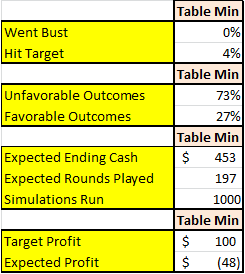
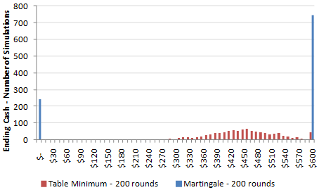
It should be no surprise that someone betting the table minimum for 200 rounds is likely to lose money on a table where the house has an edge, and we find a 73% chance that he will lose money. Charting the outcomes, you can see a classic bell curve in which he is expected to lose $47, and unlikely to lose more than $150 (7.5% in this simulation).
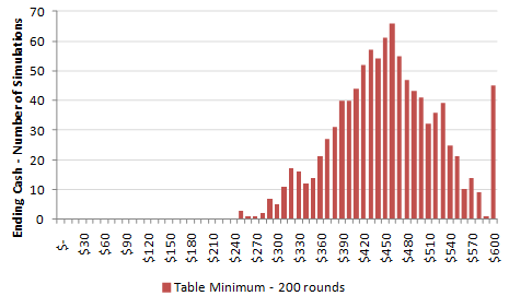
There is an apparent pile-up at $600, which is the target gain for the player. Although it is one of the more likely outcomes, it makes up only a 4.5% chance. In other words, the player faces a 95% chance of not reaching his goal. Thus, the table minimum strategy could be called "Get poor slowly".
Changing the rounds played from 200 to 500 has two main impacts. The expected loss more than doubles to $125, and the bell curve becomes less peaked. In nerd speak, the outcomes become more dispersed. In plain English, you can expect a wider range of outcomes, and the average outcome becomes less likely. More time to gamble means more time for your cash position to change.
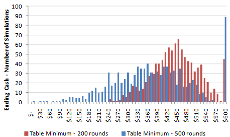
Interestingly, you are twice as likely to hit your goal by playing longer, and it becomes the most likely scenario (although still less than 1 in 10). However, you also have a higher chance of losing: 84%.
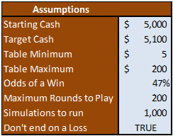
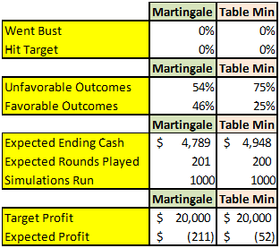
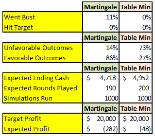
The simulator compares a Martingale strategy to this simple table minimum strategy under a set of assumptions. Here are the default set of rules:
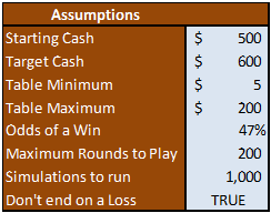
They are all pretty straightforward, other than "Don't end on a Loss". This applies to the Martingale Strategy. If, for instance, you reach the 200th round and you have lost 4 consecutive bets, you would not walk away. Instead, you would keep playing until you either win a bet or lose all of your money.
On the left side of the file, it will simulate using the strategy 1,000 times. On the right side, it will simulate simply betting the table minimum for the same number of rounds. One way to measure outcomes is to look at the percentage of simulations in which the player ends with more money than he began with. Here the Martingale strategy is the clear winner:
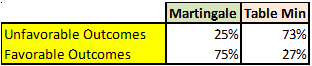
There is a 3 in 4 chance that a Martingale player will walk away richer than he began, while a player betting the table minimum has almost the same odds of walking away poorer. It seems pretty cut and dry: the Martingale strategy is much more likely to lead to an increase in cash.
A deeper examination, however, brings up an issue:
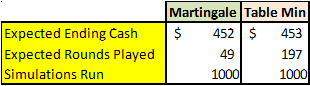
This box tells us that, on average, the Martingale player will expect to end with $452, down $48 from where he began and slightly behind the table minimum player. This is simply the average of the ending cash in each of the 1000 simulations. If the Martingale player has a 3 in 4 chance of winning, how could his expected outcome be negative?
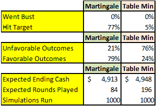
Consider a third measure of outcome: the probability that the player will go bust and lose all of his money. Here, we see another story:
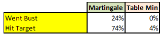
Under this set of assumptions, the Martingale player has a 1 in 4 chance of losing all of his $500 in starting cash. That means that nearly all of the unfavorable outcomes in a Martingale Strategy are a complete loss, and nearly all of the favorable outcomes are when the player makes his target.
The Table Minimum player, meanwhile, is quite unlikely to hit his target (in this case an increase of $100, or 20 minimum bets). However, he is almost certain not to lose all of his money. In this particular set of 1000 simulations, he does not go broke a single time.
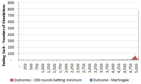
This time, the histogram puts it starkly:
The Martingale Strategy is a pure feast-or-famine in which only extreme outcomes are likely. While the table minimum player has a good expectation of where he will end up (a 79% chance he will have no more than a $100 change from where he started), the Martingale player is likely to either reach his goal or go bust. There is only a 0.6% chance he will end up less than $100 different from where he began. Notice that the table minimum player will come within 20% of the expected outcome ($452) 18% of the time, while the Martingale player will fall into the same range one tenth of 1% of the time.
Here the difference between the two strategies is pretty easy to see. Let's begin to relax some of the starting assumptions. First, let's increase the starting cash by 10x to $5000. That gives the player 1000 times the minimum bet.
Under these assumptions, we see very similar outcomes. The Martingale player comes out favorably in 77% of simulations, but still has a lower expected outcome. However, the probability of losing all of his money drops to near zero.
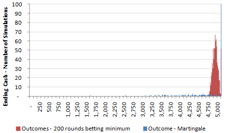
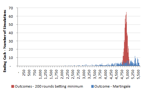
To capture this variation, we really need to look at the same histogram 3 times with different scales. The first shows the overall view:
The minimum player gets his normal bell curve that peaks $50 south of where he started. The Martingale player, again, has an enormous peak at the target of $5100. The rest of his outcomes are nearly invisible at this resolution. Dropping the vertical scale to 100 gives us a better idea of the table minimum player:
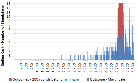
The Martingale player's outcomes are still out of focus. Dropping the scale again to 5 gives us this view:
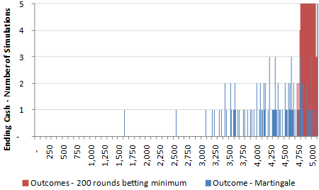
The Martingale story now begins to make sense. 77% of the time, the player does not hit a bad streak and reaches his goal, advancing in small movements. However, in the remaining 23% of cases, he loses one or more maximum bets of $200, which takes his money down significantly. In one case he loses half of his starting $5k, and in another he loses two thirds of it. Because he is limited by time, he does not always make up the ground from a bad run.
The next assumption to relax is the target cash. We have been assuming that a player will walk away once he hits his target, and that this target is a $100 return on a base investment of $5k. The Martingale player has been expecting to play 84 rounds, but he may be finished in only 27. This could be an hour in the casino, and he would have nothing left to do. Increasing the target to 25k effectively removes its effect.
Under this scenario, there is a dramatic shift in the results:
While the table minimum player is unaffected, the Martingale player is now expected to lose four times as much money overall. His odds of walking away a winner have dropped from 77% to 46%. His average outcome has dropped too, although his average outcome should not be confused with his typical outcome.
Again, the first scale shows us the table min player. Removing the target means that he no longer stops at $5100, and gets the normal curve's tail on the high end that is similar to what he has on the low end. His maximum profit in this simulation is only $160.
We see a wider array of outcomes for the Martingale player. They are no longer piling up at $5100, and his favorable outcomes extend to nearly $5600. There appear to be a few peaks, but they are very low and do not stay consistent if you run the simulation multiple times.
Next, let's adjust the table maximum. Rather than capping it at $200, we will increase it to $5000. While you are unlikely to find a table with these sorts of rules, it's worth simulating to learn why that is true.
Raising the table maximum has a dramatic effect on the outcome. The first, and most notable change, is that the Martingale player can now expect a favorable outcome 86% of the time. That means the change made him nearly twice as likely to walk away a winner as the previous set of assumptions. However, we also see an increased likelihood of losing all of his money.
This the next lesson of the Martingale strategy – a higher table maximum both helps and hurts the player by making more extreme outcomes likely.
This time, the martingale player appears to have a nice bell curve that centers around $5400. However, the 11% chance of going bust shows up all the way at zero. There are also a handful of other outcomes showing heavy losses where the player ends round 200 with less than $1000 remaining. These are likely simulations in which the player was about run out of money, but ran out of time first.
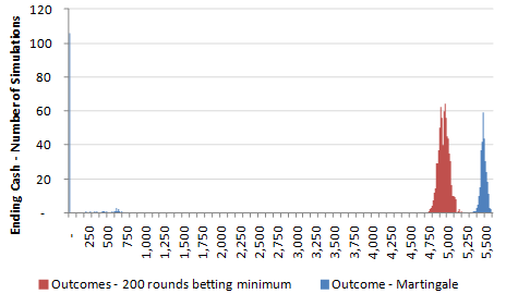
The story is pretty clear here. The Martingale strategy is working well, except for when the player hits a bad streak of luck. Eight out of ten times, the player will earn a nice, reliable return. But in the remaining simulations, his bet continues to escalate as the consecutive losses mount. The obvious strategy then is to begin with a larger cushion to insure against a bad streak. The next simulation increases the beginning cash to $20k, still at a table with a $5 minimum.
Under these assumptions, the Martingale strategy is going to be successful 93% of the time, and the risk of going broke has dropped to 2%. However, this risk is now much greater: we are now speaking of losing $20k, or 4 times as much money. That means the expected outcome is still below the minimum bet player:

However, the Martingale player has a much worse profile. Extending playing time by 10x actually increased his expected losses by 15x, and he now has more than a 1 in 5 chance of suffering a catastrophic loss. The only difference between this scenario and the last one is total playing time. Remember, we are speaking of a player entering the game with 4,000 times the minimum bet, and the Martingale system provides a strong risk of losing all of his money.
This histogram is particularly interesting:
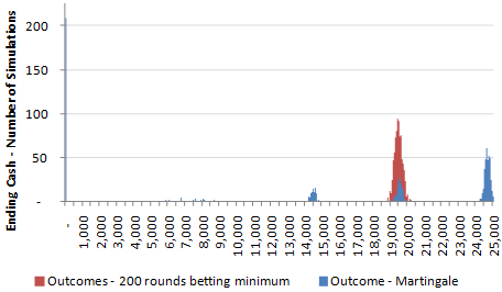
We see four distinct clusters in the Martingale strategy. From right to left, the first is near $25k. This accounts for nearly half of the simulations, and represents scenarios when the player never hit a streak of bad luck. Too put it more exactly, he did not lose more than 11 consecutive hands, or enough to reach the table maximum.
On his 11th bet, the player will have escalated his wager to $5k, which would be $5120 if the table allowed. This can be calculated as 5*(2^10). If he loses this hand, he will lose another $5k, but he will not be able to double his next bet.
This explains the cluster near $20k. These are simulations in which the player lost that 11th hand, and then won the 12th hand, recovering a max bet. If he were unconstrained, he would have wagered $10,240 and climbed back to where he started. Players in this cluster spend most of the two thousand rounds inching upwards $10 at a time, until they hit a sudden $5k drop. They have enough money to absorb the single loss, but it wipes out all of their gains.
The next cluster is near $15k. These are simulations in which the player lost the 12th consecutive hand or, even worse, lost 11 consecutive hands twice. The player here walks away losing approximately one maximum bet.
The next cluster is small and a bit more fragmented, but ranges from $5k to $9k. This represents a combined total loss of 2 or 3 max bets. It may be obtained by losing 13 consecutive bets, or some other permutation (for instance losing 12 consecutive bets, recovering, and then later losing another 11 consecutive bets).
The final cluster is the familiar scenario of the player being wiped out, and accounts for 21% of the simulations. Again the player could arrive here through a number of scenarios, but it is likely that a single bad run devastated him, handing him 14 consecutive losses.

This illustrates the core results of the Martingale strategy. It takes a relatively simple game - one in which you can expect to lose money, but in a slow and predictable way – and replaces it with a much more complex and risky one. You have a good shot at walking away a winner, but may lose your entire bankroll in a small number of rounds. One simulated player in the above chart lost his $20,000 in 20 rounds, which would take less than an hour.
Another finding from this series of simulations is that the house edge was not erased under any set of assumptions. Note that the ‘Expected Profit’ in each of tables is lower for the Martingale strategy. While the majority of players using the strategy will walk away winners, more than enough will lose their entire bankroll to offset the losses. I wouldn’t be surprised if casino operators are among those advocating the strategy. While the Martingale Strategy appears to lower risk because of its high probability of a positive outcome, it actually just shifts the risk into a small number of complete losses.
The final result from these simulations is that the outcome is dependent upon a dynamic interplay between the player’s starting cash, the table maximum, and the amount of time the player is willing to play. Simplistic advice about how much money you need to “safely” apply the strategy should be ignored. Folk wisdom will say that you will be okay with (for instance) 100 times the minimum bet. The only thing that makes the Martingale strategy safe is a low table maximum, which forces the player to abandon the strategy when consecutive losses get out of hand. The Martingale strategy can lull a player into a false sense of security by providing modest profits the first few times he uses it, only to wipe out all of those gains and more on a subsequent gambling trip.
This wraps up part 2. Click here to continue on to part 3, What the Martingale Strategy Can Teach us about Debt.